SQL Recursive CTE queries in are commonly used when working with hierarchical data in Relational Databases. For e.g. the following Highway Network:
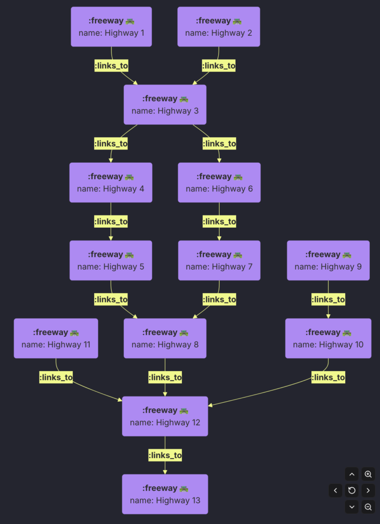
Let’s say we are interested in getting all the path from each Highway to other Highways. We would use a Recursive CTE for that. Let’s create some sample data and write a Recursive CTE Queries to extract all the PATHs.
create table flows_to (
    highway_from varchar(100)
    , highway_to varchar(100)
);

insert INTO FLOWS_TO (highway_from, highway_to) VALUES
(null, 'highway_1'), -- starting node
(null, 'highway_2'), -- starting node
(null, 'highway_9'), -- starting node
(null, 'highway_11'), -- starting node
('highway_1', 'highway_3'),
('highway_2', 'highway_3'),
('highway_3', 'highway_4'),
('highway_3', 'highway_6'),
('highway_4', 'highway_5'),
('highway_6', 'highway_7'),
('highway_7', 'highway_8'),
('highway_5', 'highway_8'),
('highway_9', 'highway_10'),
('highway_10', 'highway_12'),
('highway_8', 'highway_12'),
('highway_11', 'highway_12'),
('highway_12', 'highway_13');Now let’s construct a Recursive CTE for this:
WITH  outcome(starting, highway_to, highway_from, path) AS (

  -- ANCHOR: Initial query to establish the base result set.
  SELECT -- Anchor
    highway_to as starting
    , highway_to
    , highway_from
    , highway_to as path
  FROM flows_to
  WHERE highway_from is null

  UNION ALL

  -- RECURSIVE: References outcome CTE to build on previous results
  SELECT starting, flows_to.highway_to, flows_to.highway_from, outcome.path || '->' || flows_to.highway_to
  FROM outcome
  JOIN flows_to ON flows_to.highway_from = outcome.highway_to
)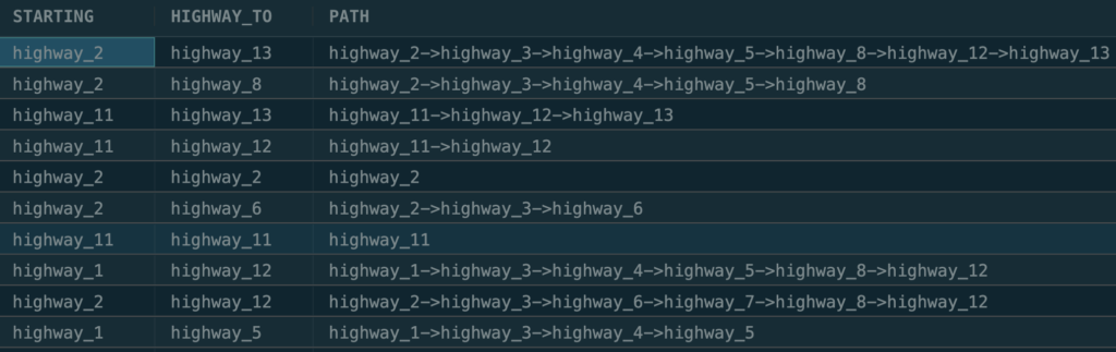
SELECT DISTINCT starting, highway_to, path FROM outcome;The above query will output:
While the recursive CTE is not complex, it is not trivial to write.
Enter GQL.
Hierarchical data is a Graph. As such a Graph Query Language (GQL) may be a more elegant way to extract the above Paths. GQL, like SQL, is a high-level, declarative, programming language. It is specifically designed for graph structures. It uses nodes and relations as first-class citizens, although the output to a query can be a graph or a set of tuples.
Let’s explore using the same dataset and query using GQL. We will start with generating sample data
drop graph freeways;
create graph freeways{
  node freeway ({name string})
  , edge flows_to (freeway)-[]->(freeway)
};


use freeways;
INSERT (n1:freeway {_id:'highway_1', name:"Highway 1"})
  , (n2:freeway {_id:'highway_2', name:"Highway 2"})
  , (n3:freeway {_id:'highway_3', name:"Highway 3"})
  , (n4:freeway {_id:'highway_4', name:"Highway 4"})
  , (n5:freeway {_id:'highway_5', name:"Highway 5"})
  , (n6:freeway {_id:'highway_6', name:"Highway 6"})
  , (n7:freeway {_id:'highway_7', name:"Highway 7"})
  , (n8:freeway {_id:'highway_8', name:"Highway 8"})
  , (n9:freeway {_id:'highway_9', name:"Highway 9"})
  , (n10:freeway {_id:'highway_10', name:"Highway 10"})
  , (n11:freeway {_id:'highway_11', name:"Highway 11"})
  , (n12:freeway {_id:'highway_12', name:"Highway 12"})
  , (n13:freeway {_id:'highway_13', name:"Highway 13"})
  , (n1)-[:flows_to]->(n3)
  , (n2)-[:flows_to]->(n3)
  , (n3)-[:flows_to]->(n4)
  , (n3)-[:flows_to]->(n6)
  , (n4)-[:flows_to]->(n5)
  , (n6)-[:flows_to]->(n7)
  , (n5)-[:flows_to]->(n8)
  , (n7)-[:flows_to]->(n8)
  , (n9)-[:flows_to]->(n10)
  , (n11)-[:flows_to]->(n12)
  , (n8)-[:flows_to]->(n12)
  , (n10)-[:flows_to]->(n12)
, (n12)-[:flows_to]->(n13);Next let’s write a GQL query to extract all the PATHs. Note that in the case of GQL, to compute and list the paths, it suffices to write:
MATCH nodes = (a)
CALL {
  MATCH path = (a)-[edges:flows_to]->{0,}(b)
  return reduce(path = a._id, edge in edges | path || '->' || edge._to) as route
  , b
}
return table(a.name, b.name, route);This will output
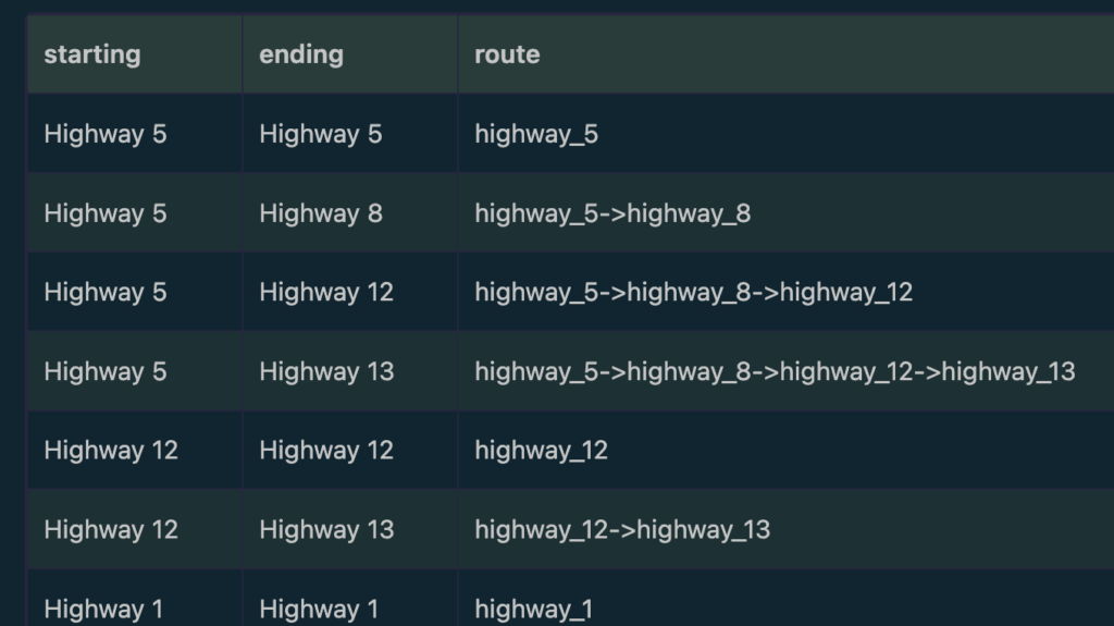
It can be seen that the structure of the GQL query is far less complicated and more intuitive than its SQL counterpart, since it takes advantage of the graph structure. In this case, a basic MATCH.. RETURN structure suffices to express a recursive query. This is mainly because GQL is developed as a query language for
graphs and recursion is typical in these cases. The(a:highway)-[:flows_to]->{0,}(b:highway) path pattern selects all nodes b that are reachable by following one or more edges in the graph, traversing the graph using the :flows_to relation.
Path patterns describe multi-hop relationships in the graph:
{2,4}: Exactly 2 to 4 hops
{0,}: 0 or more hops (unbounded)
{,3}: Up to 3 hops
{5}: Exactly 5 hops
SQL CONNECT BY clause.
Some SQL based databases support CONNECT BY Clause. This clause allows queries on hierarchical data without the need for composing complex recursive CTEs. For e.g. the following CONNECT BY clause query will find all the paths from each to all others nodes
SELECT
    level,
    highway_from,
    SYS_CONNECT_BY_PATH(highway_from, '->') || '->' || highway_to  AS path,
    highway_to
FROM
    FLOWS_TO
START WITH
    highway_from IS NULL
CONNECT BY
PRIOR highway_to = highway_from;While this query is easier to read than its recursive CTE counterpart, it is not intuitive as GQL…
Leave a Reply to Saqib Ali Cancel reply